This tutorial gives you a quick tour of the workflow and features that bossanova provides for estimating a variety of models through a single unified model class that works the same no matter what type of model you’re working with:
| Model Type | Syntax | R equivalent |
|---|---|---|
| linear | model("y ~ x") | lm(y ~ x) |
| generalized linear | model("y ~ x", family="binomial") | glm(y ~ x, family=binomial) |
| linear mixed/multi-level | model("y ~ x + (1 | x)") | lme4::lmer(y ~ x + (1 | x)) |
| generalized mixed/multi-level | model("y ~ x + (1 | x)", family="binomial") | lme4::glmer(y ~ x + (1 | x), family=binomial) |
bossanova is also tightly integrated with polars DataFrames and seaborn FacetGrids. It also includes several built-in datasets for teaching and demonstration purposes. Let’s load one now to walkthrough basic usage.
import polars as pl
from polars import col
import seaborn as sns
from bossanova import load_dataset
credit = load_dataset("credit")
credit.head()Overview
Methods
| Name | Description |
|---|---|
fit() | Fit the model to data. |
simulate() | Generate data from scratch or simulate responses from a fitted model. |
predict() | Generate predictions from the fitted model. |
explore() | Compute marginal effects or estimated marginal means (EMMs). |
infer() | Augment current results with statistical inference. |
summary() | Generate a formatted model summary (R-style or compact). |
Attributes
| Attribute | Type | Available after | Description |
|---|---|---|---|
designmat | pl.DataFrame | model creation | Fixed-effects design matrix as a named DataFrame. |
metadata | pl.DataFrame | model creation | Meta-data about missing observations |
params | pl.DataFrame | .fit() | Coefficient estimates table from the fitted model. |
diagnostics | pl.DataFrame | .fit() | Model-level goodness-of-fit diagnostics. |
effects | pl.DataFrame | .explore() | Marginal effects or estimated marginal means (EMMs) table. |
predictions | pl.DataFrame | .predict() | Predictions table from the fitted model. |
simulations | pl.DataFrame | .simulate() | Simulations table from data generation or response simulation. |
resamples | pl.DataFrame | None | .infer() | Raw resampled values from bootstrap or permutation inference. |
1. Universal model class
A model that needs at least two arguments:
formula: a string specifying the model using Wilkinson notation (same as R’s
lm/glm/lmer/glmer)data: a polars DataFrame (optional if you just want to simulate)
# Import model
from bossanova import model

# Create one
m1 = model("Balance ~ Income * Student", credit)

# Check it out
m1The design matrix
Before fitting, we can inspect the design matrix — the actual numbers the model will work with. This is the matrix from the GLM equation :
m1.designmat.head()Visualizing it can be extremely helpful to ensure estimates are what you intended when fitting:
# seaborn facetgrid kwargs are supported
m1.plot_design()
m1.plot_design(aspect=2)
<seaborn.axisgrid.FacetGrid at 0x1080081a0><seaborn.axisgrid.FacetGrid at 0x15efc1450>

The design matrix has one row per observation and one column per model term:
Intercept — a column of 1s (the “constant” that captures the baseline level of Balance)
Income — the raw income values for each person
Student — a categorical factor with treatment coding and 2 levels
Income:Student — the interaction term
Multi-collinearity & variance inflation
Before fitting a model we can inspect how much multi-collinearity between predictors might inflate our uncertainty:
m1.plot_vif()<seaborn.axisgrid.FacetGrid at 0x15eff3b10>
Factors & transformations
Since we’re including an interaction it’s helpful to center Income. bossanova supports all kinds of transformations directly in the formula
# Center Income and use sum/deviation coding for Student
m1 = model("Balance ~ center(Income) * Student", credit)

# See new VIF
m1.plot_vif()
<seaborn.axisgrid.FacetGrid at 0x15f3e3110>
Given the tight integration with polars which requires each column of a dataframe to have the same type, bossanova will automatically treat all non-numeric columns as factors using a default treatment/dummy coding scheme with the reference level as the first alphabetical level:
m2 = model("Balance ~ Ethnicity", credit)
m2.plot_design()
<seaborn.axisgrid.FacetGrid at 0x15f3e2d50>
We can adjust this by specifying the coding scheme directly in the formula:
m2 = model("Balance ~ poly(Ethnicity)", credit)
m2.plot_design()
<seaborn.axisgrid.FacetGrid at 0x15f861bd0>
Formula reference
Also available in the model API reference.
Operators
| Operator | Example | Meaning |
|---|---|---|
+ | a + b | Main effects (additive) |
* | a * b | Main effects + interaction (a + b + a:b) |
: | a:b | Interaction term only |
** / ^ | x**2 | Power term (quadratic, cubic, etc.) |
| | (1 | group) | Random effect (mixed models) |
In-formula transforms
| Transform | Effect | Example |
|---|---|---|
center(x) | x - mean(x) | y ~ center(age) |
norm(x) | x / sd(x) | y ~ norm(income) |
zscore(x) | (x - mean(x)) / sd(x) | y ~ zscore(x) |
scale(x) | (x - mean(x)) / (2 * sd(x)) — Gelman scaling | y ~ scale(x) |
rank(x) | Average-method rank | y ~ rank(x) |
signed_rank(x) | sign(x) * rank(|x|) | y ~ signed_rank(x) |
log(x) | Natural log | y ~ log(x) |
log10(x) | Base-10 log | y ~ log10(x) |
sqrt(x) | Square root | y ~ sqrt(x) |
poly(x, d) | Orthogonal polynomial basis of degree d | y ~ poly(x, 2) |
factor(x) | Treat as categorical | y ~ factor(year) |
All stateful transforms (center, norm, zscore, scale, rank, signed_rank) learn parameters from training data and reapply them on new data during .predict(). Nesting is supported: zscore(rank(x)).
Contrast coding (in-formula)
| Function | Example | Intercept means | Coefficients mean |
|---|---|---|---|
treatment(x) | y ~ treatment(group) | Reference level mean | Difference from reference |
sum(x) | y ~ sum(group) | Grand mean | Deviation from grand mean |
helmert(x) | y ~ helmert(group) | Grand mean | Level vs. mean of previous levels |
poly(x) | y ~ poly(group) | Grand mean | Linear, quadratic, cubic trends |
sequential(x) | y ~ sequential(group) | First level mean | Successive differences (B-A, C-B) |
Set a custom reference level or ordering with keyword args: treatment(group, ref=B), sum(group, omit=A), helmert(group, [low, med, high]).
model("y ~ sum(group) + x", data)                    # sum coding
model("y ~ treatment(group, ref=B) + x", data)       # treatment with ref="B"
model("y ~ group + x", data, contrasts={"group": M}) # custom ndarray matrix
2. .fit(): model estimation
To estimate the model parameters (), we can call .fit()
Parameter estimates
This returns parameter estimates as a dataframe in also accessible in .params
m1.fit()Model diagnostics
The .diagnostics property gives us key fit statistics:
m1.diagnosticsWe can also check the .metadata which summarizes useful info about the data the model use for fitting. This is helpful because we have to drop rows where data is missing and this lets you inspect if/when that’s happening.
m1.metadatamodels also include a variety of plotting methods to inspect the model fit and errors:
m1.plot_resid()<seaborn.axisgrid.FacetGrid at 0x15f9cde50>
Augmented fits & predictions
Similar to libraries like broom in R, after calling .fit(), the .data property of a model stores the original data plus several computed columns:
| Column | Description |
|---|---|
fitted | Predicted values () |
resid | Residuals () |
hat | Leverage values |
std_resid | Standardized residuals |
cooksd | Cook’s distance (influence) |
m1.data.head()Let’s plot predicted vs observed Balance to see how well our model does:
sns.relplot(
    data=m1.data.to_pandas(),
    x="fitted",
    y="Balance",
    kind="scatter",
    height=4,
    aspect=1.2,
).set_axis_labels("Predicted Balance", "Observed Balance")
<seaborn.axisgrid.FacetGrid at 0x15dba11d0>
3. .infer(): uncertainty & inference
Asymptotic (default)
m1.infer()sleep = load_dataset("sleep")
lmm = model("Reaction ~ Days + (Days | Subject)", sleep).fit()
lmm.infer()Bootstrap resampling
m1.infer(how="boot")Bootstrap inference resamples the data with replacement, refits the model each time, and builds confidence intervals from the empirical distribution of estimates. By default it uses bias-corrected and accelerated (BCa) intervals with 1000 resamples. Control the number with n_boot=:
m1.infer(how="boot", n_boot=2000)The raw bootstrap distributions are stored in .resamples and can be visualized:
m1.plot_resamples()<seaborn.axisgrid.FacetGrid at 0x168be0410>
Permutation resampling
m1.infer(how="perm")4. .jointtest(): omnibus (ANOVA) tests
While .infer() tests each coefficient individually, .jointtest() performs ANOVA-style omnibus F-tests that ask whether an entire predictor (which may span multiple coefficients, like a multi-level factor or an interaction) explains significant variance:
m1.jointtest()5. .explore(): marginal effects
.explore() computes estimated marginal means (EMMs) for categorical predictors and marginal slopes for continuous ones. It uses an R-style formula mini-language to specify what you want to see. Let’s switch to the Titanic dataset and fit a logistic regression to see how survival depends on sex, age, and their interaction:
titanic = load_dataset("titanic")
m2 = model("survived ~ sex * age", titanic, family="binomial").fit()
m2.infer()For a categorical predictor, .explore() returns the model-predicted mean at each level; for a continuous predictor, it returns the average slope (rate of change):
# EMMs for sex — predicted survival probability for each level
m2.explore("sex")# Marginal slope of age — average rate of change in survival per year
m2.explore("age")Focal exploration with @
The @ operator pins a variable at specific values. Use it to evaluate the model at chosen points rather than the default grid:
# Survival slope at specific ages
m2.explore("age@[20, 40, 60]")# EMM for a single sex level
m2.explore("sex@female")Conditional exploration with ~
The ~ operator breaks results out by another variable, letting you see how effects differ across groups or values of a moderator:
# How does the age slope differ between men and women?
m2.explore("age ~ sex")Contrasts
Compute contrasts directly using bracket notation or named contrast functions:
# Difference in survival between males and females
m2.explore("sex[male - female]")# Pairwise with inference
m2.explore("pairwise(sex)").infer()Visualizing with .plot_explore()
.plot_explore() accepts the same formula syntax and produces a seaborn FacetGrid:
m2.plot_explore("age ~ sex")<seaborn.axisgrid.FacetGrid at 0x374176210>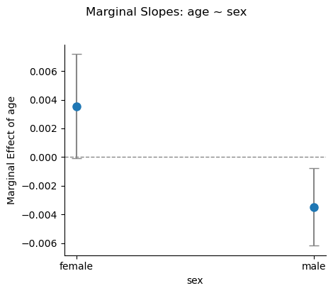
m2.plot_explore("sex")<seaborn.axisgrid.FacetGrid at 0x3743ec190>
Cheatsheet
Also available in the explore API reference.
| Formula | Computes |
|---|---|
"X" | EMMs (categorical) or marginal slope (continuous) |
"X@v" | EMM at a single value |
"X@[a, b, c]" | EMMs at specific levels or values |
"X@range(n)" | EMMs at n evenly-spaced values |
"X@quantile(n)" | EMMs at n quantile values |
"X ~ Z" | Break X out by levels of Z |
"X ~ Z@v" | Pin Z at value v |
"X ~ Z@[v1, v2]" | Cross X with multiple Z values |
"X ~ Z@range(n)" | Cross X with n evenly-spaced Z values |
"X ~ Z@quantile(n)" | Cross X with n quantile Z values |
"X ~ A + B" | Multiple conditions |
X[A - B] | A minus B |
X[A - B, C - B] | Multiple comparisons |
X[* - B] | Each other level vs B |
X[(A + B) - C] | mean(A, B) minus C |
X[A - B] ~ Z[C - D] | Interaction: (A-B at C) minus (A-B at D) |
x ~ Z[A - B] | Slope of x at A minus slope at B |
X:Z[A:C - B:D] | Cell A:C minus cell B:D |
Functions for specific contrasts:
| Formula | Computes | Order-dependent |
|---|---|---|
treatment(X, ref=A) | Each level vs reference A | No |
dummy(X, ref=A) | same as treatment | No |
sum(X) | Each level vs grand mean | No |
deviation(X, ref=A) | same as sum | No |
poly(X) / poly(X, d) | Orthogonal polynomials up to degree d | Yes |
sequential(X) | Adjacent: B-A, C-B | Yes |
helmert(X) | Each level vs mean of previous | Yes |
pairwise(X) | All pairs: B-A, C-A, C-B | No |
Effects scaling control:
| Kwarg | Values | Effect |
|---|---|---|
effect_scale | "auto" (default), "link", "response" | "auto" = "response" for AME/GLM, "link" otherwise |
varying | "exclude" (default), "include" | Population vs group-specific (mixed models) |
inverse_transforms | True (default), False | Auto-resolve center(x) / zscore(x) |
6. .predict(): generalization
.predict() generates predictions from the fitted model. It accepts a formula string, a DataFrame, or None:
# Predictions on training data
m2.predict()Formula-mode predictions
Pass a formula string to build a prediction grid automatically — like R’s ggpredict(). Grid columns are prepended to the output:
# Predicted survival across ages, broken out by sex
m2.predict("age ~ sex")The same @ modifiers from .explore() work here too:
# 10-point age grid crossed with sex
m2.predict("age@range(10) ~ sex")Chain .infer() to add confidence intervals to the grid:
m2.predict("age ~ sex").infer()DataFrame predictions
Pass a DataFrame to predict on specific new observations:
new_passengers = pl.DataFrame({"sex": ["male", "female", "male"], "age": [25.0, 40.0, 60.0]})
m2.predict(new_passengers)Visualizing with .plot_predict()
.plot_predict() accepts the same formula syntax and produces a seaborn FacetGrid showing predicted trends with confidence bands:
m2.plot_predict("age ~ sex")<seaborn.axisgrid.FacetGrid at 0x37434fb10>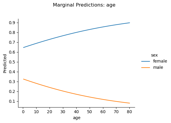
m2.plot_predict("age ~ sex", show_data=True, show_rug=True)<seaborn.axisgrid.FacetGrid at 0x3745ae210>
Cross-validated model ablation
Use .infer(how="cv") to evaluate out-of-sample prediction accuracy via k-fold cross-validation. This is useful for comparing models — a model with lower CV error generalizes better:
m2.infer(how="cv", k=5)m2.diagnostics7. .simulate(): planning
Power Analysis
from bossanova.distributions import normalm = model("y ~ x")
m.simulate(
n=100,
x=normal(0, 1),
coef={"x": 0.5},
sigma=1.0,
power=500,
)
m.power_resultsEach row corresponds to one model parameter (here, Intercept and x):
| Column | Meaning |
|---|---|
| n | Sample size used |
| term | Parameter name |
| true_value | The true coefficient you specified (0 for unspecified terms) |
| power | Proportion of simulations where the p-value < 0.05 |
| power_ci_lower/upper | Wilson score 95% CI on the power estimate |
| coverage | Proportion of 95% CIs that contain the true value (~0.95 if well-calibrated) |
| bias | Mean estimate minus true value (should be near 0) |
| rmse | Root mean squared error of estimates |
| mean_se | Average estimated standard error |
| empirical_se | Standard deviation of estimates across simulations |
| n_sims | Number of successful simulations |
| n_failed | Number of simulations that failed to converge |
For the Intercept (true value = 0), “power” is really the Type I error rate — it should be around 0.05. For x (true value = 0.5), power tells you how often you’d correctly reject .
power=500 means “run 500 simulations.” Each simulation generates a fresh dataset from your DGP, fits the model, and runs inference. The results are then aggregated into the power table.
Sweeping Sample Size
The most common power analysis question is: how large does my sample need to be? Pass a list of sample sizes via power={"n": [...]}:
m = model("y ~ x")
m.simulate(
    n=100,
    x=normal(0, 1),
    coef={"x": 0.3},
    sigma=1.0,
    power={"n_sims": 500, "n": [30, 50, 100, 200, 500]},
)
m.power_results.filter(m.power_results["term"] == "x").select(
    ["n", "power", "power_ci_lower", "power_ci_upper"]
)Now you can see exactly where power crosses 80% — the conventional threshold for adequate power.
Sweeping Effect Size
Sometimes you’re less sure about the effect size than the sample size. You can sweep over coefficients to see how sensitive your design is:
m = model("y ~ x")
m.simulate(
    n=100,
    x=normal(0, 1),
    coef={"x": 0.3},
    sigma=1.0,
    power={"n_sims": 500, "coef": {"x": [0.1, 0.2, 0.3, 0.5, 0.8]}},
)
m.power_results.filter(m.power_results["term"] == "x").select(
    ["true_value", "power", "coverage", "bias"]
)With , a small effect () is nearly undetectable, while a large effect () is found almost every time. Coverage should stay near 0.95 regardless of effect size — that’s a sign the inference is well-calibrated.
Full Factorial Sweeps
You can sweep multiple axes simultaneously. bossanova takes the full Cartesian product:
m = model("y ~ x")
m.simulate(
    n=50,
    x=normal(0, 1),
    coef={"x": 0.3},
    sigma=1.0,
    power={
        "n_sims": 300,
        "n": [50, 100, 200],
        "coef": {"x": [0.2, 0.5]},
    },
)

# Filter to x and show the power surface
m.power_results.filter(
    m.power_results["term"] == "x"
).select(["n", "true_value", "power"])This gives you a 3 × 2 = 6-row power surface: for each combination of sample size and effect size, you see the estimated power. This is exactly the kind of table you’d include in a grant application or pre-registration.
Tips
Choosing n_sims: More simulations give tighter power estimates (the Wilson CIs shrink). 500 is a good default; 1000+ for final reports. For quick exploration, 100–200 is fine.
Interpreting coverage: If coverage is substantially below 0.95, your model’s confidence intervals are too narrow (anti-conservative). This can happen with very small samples or misspecified models.
Bias and RMSE: Bias should be near zero for well-specified models. RMSE combines bias and variance — it shrinks as increases.
Multiple predictors: Power analysis works with any formula. Each parameter gets its own row in the results:
8. compare(): model comparison
bossanova provides compare() as a general purpose model comparison function. You can use this to compare nested and non-nested models with a variety of approaches:
from bossanova import comparem0 = model("Balance ~ 1", credit).fit()
m1 = model("Balance ~ Income", credit).fit()
compare(m0, m1)Compare varying (random) effect structures for mixed-models:
sleep = load_dataset("sleep")

intercept_only = model("Reaction ~ Days + (1 | Subject)", sleep).fit()
intercept_slope = model("Reaction ~ Days + (Days | Subject)", sleep).fit()
compare(intercept_only, intercept_slope)